Blog by: Joe Marion
Forward: This post is about the continual reassessment method, a type of design used for phase I dose-finding studies, particularly in oncology. These designs use statistical models to make sequential decisions about how to allocate patients to doses of a drug with an unknown safety profile. The goal is to determine the MTD, the largest dose at which the probability of a safety event (usually a dose-limiting toxicity) occurs with probability less than ρ*. Bayesian methods are common for these designs for the simple reason that these decisions are made with minimal evidence – prior information is crucial to obtaining reasonable model estimates, which in turn lead to favorable operating characteristics. For an overview of these designs, I’d recommend the book “Dose finding by the Continual Reassessment Method” by Cheung (2011) or the chapter on Phase I studies from “Bayesian Adaptive Methods for Clinical Trials” by Berry et al. (2010).
Phase I dose-escalation designs pose a unique challenge for statisticians: how do we make decisions in an environment of limited data? The stakes are often high, as many of these trials are first-in-human, and there is limited knowledge about the safety profile of a new drug. Good designs need to balance the desire to escalate to higher, potentially more efficacious doses with the imperative to safeguard patients and limit exposure to unnecessary toxicity.
Bayesian designs approach this challenging problem by incorporating expert scientific and clinical information into a design in the form of prior information. At which doses are toxicities anticipated? Will the toxicity of the drug rise quickly, or do we expect a more gradual increase? This knowledge can be included in a CRM through the choice of a prior distribution. A well-chosen prior distribution leads to a design that reacts more appropriately to the data, providing an appropriate tradeoff between exploring higher doses and preserving patient safety. The challenge in designing a Bayesian dose-escalation is that the ‘right’ prior is different for every trial, and finding a good choice takes substantial effort.
In this post, I’m going to discuss why choosing a prior is difficult and suggest a straightforward solution to make these trials easier to design. I focus on model-based designs like the continual reassessment method (CRM) and Escalation with Overdose Control (EWOC). The key idea is that we can choose a better prior distribution by changing our model so that it has a more intuitive interpretation. Rather than working with abstract statistical parameters, we can simplify the design process by working directly with parameters that have a straightforward clinical interpretation.
A Prior Problem
One of my favorite things about designing a CRM is that they feel properly Bayesian. The prior information plays a really important role here because the data are generally limited. Imagine that you need to estimate the probability of a safety event on a dose with only one patient’s worth of data. Would you be satisfied with the empirical estimate of either 0% or 100%? How would you quantify the uncertainty in that estimate?
A good prior distribution can be helpful in this situation, and the choice of prior plays an important role in determining the doses that the model recommends. Unfortunately, finding that prior is a complicated process. We like to spend lots of time working with clinicians, showing them how the model reacts to example data sets. What decisions do they like? What makes them uncomfortable? I view this as a kind of prior elicitation, using the clinician’s reaction to the model to “back into” an appropriate prior. Put another we, we try to choose a prior that pre-specifies the decisions a clinician would make if they were observing data from the actual trial. Then, when we’ve got the prior dialed in, we simulate the design under many different conditions to make sure that it has good performance.
This process works well, but it’s not easy. We spend a lot of time tweaking the prior, trying to get the behavior just right. A prior that improves behavior in one part of the dose range may behave badly in another. Or maybe the model behaves well for steep dose-response curves but escalates too slowly when toxicity increases slowly. Getting the prior right is a labor of love and requires substantial effort. The good news is that changing the way the model is parameterized greatly simplifies the prior specification.
The Two-parameter Logistic Regression
We start with a two-parameter logistic regression, which is commonly used in CRM, EWOC, and other Bayesian designs.

The parameter ρi is the probability of a safety event, xi is a dose level, α is an intercept, and β is a slope. The model is completed by placing priors on the parameters, usually with the restriction that β is positive to enforce monotonicity.
Suppose we are targeting the largest dose with a toxicity rate of 0.3 and that we have dose levels xi Ε {10,20,…,100}. The dose at which the MTD occurs depends on both parameters; the following plot shows different combinations of α and β where ρi = 0.3 by dose level.
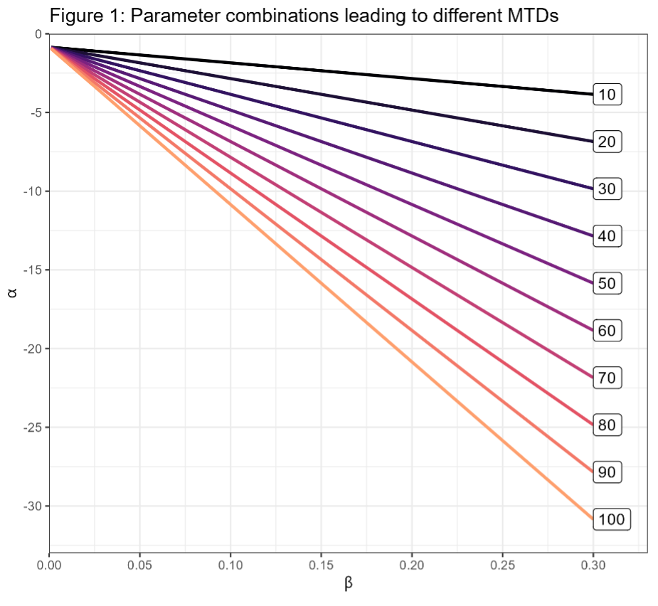
This figure is sort of a contour plot; each parameter combination along a line leads to the same dose being chosen as the MTD. The different levels of β along the line correspond to different amounts of steepness in the dose-toxicity curve. Looking at the plot, you can kind of see why these models are sensitive to the prior. When dose-toxicity relationship rises slowly (β near 0) we’d like a prior that place most of the mass near -1 (ish). On the other hand, when toxicity increases quickly ( β near 0.3) the prior for α needs to span a wide range if we’d like to each dose to have a reasonable prior probability.
Suppose you placed a Unif(0, -30) prior on α and a Unif(0, 0.3) prior on β. Here’s the prior probability of selecting each dose with this prior distribution.
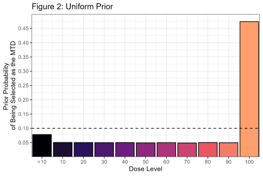
This is one of those cases where an “uninformative” prior is actually very informative. Looking at Figure 1, most of the prior mass falls in the lower-left triangle below the orange Dose=100 line. The doses where ρi = 0.3 (and thus dose i is the MTD) in this region lie above the maximum dose of 100, but 100 is the maximum for our design, and so this dose would be ‘selected’ in that region of the prior. When we choose the dose levels for a design, that decision reflects our understanding of which doses are likely to be safe. The uniform prior conflicts badly with the design; we’ve chosen 100 as our maximum dose because doses above 100 are unlikely to be safe. Unfortunately, this prior suggests the opposite. It would be difficult to get good behavior from a design where the prior distribution conflicts so strongly with the clinical expectation.
There’s another issue with this prior, which is that the prior distribution of the slope changes substantially with the prior-MTD. I’m not going to describe this problem in depth, but it further increases the difficulty of choosing a good prior because changes that positively improve the distribution of the prior-MTD have unintended impacts on the shape of the dose-toxicity relationship.
Of course, you can change the prior to get different kinds of behavior. You might change the hyperparameter or even change the family of distributions – FACTS uses a multivariate normal/log-normal. With enough fiddling you can often find something that “works,” but the process is tedious, time-consuming, and may ultimately result in a prior that is only satisfactory.
This One Weird Trick You Won’t Believe!
The problem with choosing a prior is that our prior knowledge is about things like “which dose is likely to be the MTD” or “what is the probability that the lowest dose is safe” but it’s not clear how to incorporate that kind of information using α and β. When you think about things this way, the natural solution is to re-parameterize the model so that you can place a prior distribution on the quantities that you know something about. Here’s a simple re-parameterization that places a prior on the MTD.

As a reminder, ρ* is the target DLT rate at the MTD. The parameter ϒ is the dose at which the MTD occurs. Placing a prior on ϒ is natural because you are working directly with a parameter you can interpret.
When an expert tells me “The starting dose is particularly conservative, so we don’t expect DLT’s in that region. The MTD is likely to occur near the 60-70mg dose level, but there’s some possibility that we could escalate all the way to 100” then I can easily specify a prior on ϒ with that behavior:
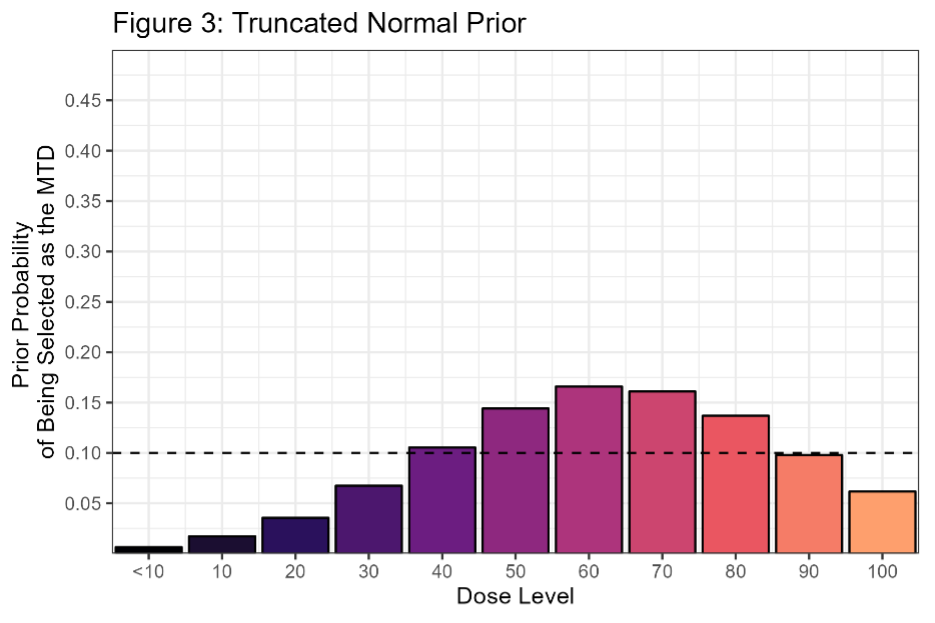
This is a normal prior truncated to (0, 110) with a mean of 65 and a standard deviation of 20. There’s still some art in getting the prior distribution right, but the process is much easier because you can intuitively understand how changing this prior would affect the design. For example, I might want to increase prior probability that all the doses are unsafe (MTD < 10). To do this, I could make the prior a mixture distribution with one of the components centered near 0. Another nice feature is that you still freedom to control the slope of the dose-response curve by varying the prior on β, and these changes don’t change the prior on the MTD. So, you can focus on changing one element at a time.

Here x0 is the smallest dose-level and 𝜋0 is the prior probability of a DLT that dose. This kind of parameterization gives you more control over the behavior of the model at the beginning of the escalation, so that you can specify how the model reacts to an early DLT. Here’s another parameterization that I’ve found useful:

For this parameterization 𝑑 < 0 is a dose increment and 𝜋+ Ε[0, ρ*) is the probability of a DLT at the dose ϒ+𝑑. Choosing 𝑑 = 10 for our example leads to a prior on probability of DLT at the dose one-level below the MTD. This answers the question: how quickly do we think toxicity will rise? If we’re close to the MTD, how likely are we to reach it if we increase one dose level? How reactive should the model be when you observe the first DLT?
Wrap-up
Re-parameterizing your model won’t make designing a dose-escalation simple; you still need to pressure test the escalation rules, look at example trials to understand how the design works, and simulate operating characteristics. But a parameterization that facilitates a natural prior will make the process easier. Having a good model with behavior that you like simplifies the design process, allowing you to develop more parsimonious designs that are ultimately more robust to unforeseen complications. And, while this this is a bit of a stretch, interpretable parameterizations allow for better collaborations because they allow us (statisticians) to directly include information from other experts.
Simplifying the design process is important because model-based designs like CRM and EWOC are often criticized for being complicated clinical trials to design. These designs often have complex escalations rules, require frequent statistical modeling to support implementation, rely on simulation to demonstrate their operating characteristics, and are sensitive to the specification of prior. Compared to straightforward, “out-of-the-box” alternatives like mTPI and BOIN designs, model-based designs require more statistical expertise to design and implement. For some Phase I trials we recommend these designs – the tradeoff in complexity just doesn’t outweigh the benefits, if any, of a more complicated design.
But sometimes we are tasked with designing a complicated dose escalation: one that adaptively randomizes among multiple dosing schedules, or that includes non-DLT safety information, or that have many dose levels. Some trials need complicated designs and so the CRM/EWOC designs are an important part of our toolkit. The good news is that when you need to design these kinds of trials, re-parameterizing the prior makes that process a little bit easier.
References
Berry SM, Carlin BP, Lee JJ, Muller P. Bayesian Adaptive Methods for Clinical Trials. Boca Raton (FL): CRC Press; 2010.
Cheung YK. Dose finding by the Continual Reassessment Method. Boca Raton (FL): CRC Press; 2011.
Winkler RL, Kadane JB, Dickey RL, Smith WS, Peters SC. Interactive Elicitation of Opinion for a Normal Linear Model. Journal of the American Statistical Association. Taylor & Francis: SSH Journals; 1980;75(4):845–854.